Welp, it’s been quite a while since I last posted about parsing a WhatsApp chat. While it was cool to get the text into a usable format, it’s time to take a look at what’s actually in there. To do this, I used R’s tidytext package. Julia Silge, the Author of tidytext, also wrote a book, Texting Mining with R, that was super helpful as I began to look at this text. Best of all, this book is available online and completely free.

To start, we need to shift this data into a format that’s better for analyzing. Silge suggests moving the data to a tidy text format that is, a table with one token per row. A token is a meaningful unit of text and in this case will be a word. This format will help us use other “tidy” tools such as dplyr or ggplot2 and tidytext’s unnest_tokens function makes tokenizing this text quite easy.

library(tidyverse)
library(tidytext)
library(stringr)
library(reshape2)
library(lubridate)
library(gridExtra)

'%!in%' <- function(x, y)
  ! ('%in%'(x, y))

data <-
  read_csv("message v2.csv")

notABro <- c("No Person", "not", "Africa")

data <- filter(data, Sender %!in% notABro)

# Tidy Text
text <- data %>%
  unnest_tokens(word, Message) %>%
  anti_join(stop_words)

text %>%
  count(word, sort = TRUE)

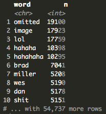
After tokenizing the text and quickly aggregating, we see that “omitted” and “image” are the most used words. When you export a WhatsApp chat, you have the option of including or excluding things like images or gifs. I chose to exclude gifs and images so instead of seeing an image or a gif, each line read “Image/Gif Ommited.” Next up we have “lol”, “hahaha”, and “hahahaha.” This is not too surprising to me since I’ve definitely been one of those people who can sit and laugh hysterically at their phone while no one else around knows what’s going on. However, it is interesting to see variations of “haha,” I began to wonder how many variations actually exist.

text %>%
  filter(str_detect(word, "haha")) %>%
  count(word, sort = TRUE)

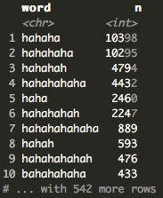
This is where having the data in a tidy format becomes helpful. We can use stringr’s str_detect to find all the “hahas.” It turns out that there are 542 variations of “haha” and the most common variation is “hahaha” followed closely by “hahahaha.” Learning this, I became curious about the longest “haha”.

text %>%
  filter(str_detect(word, "haha")) %>%
  count(word, sort = TRUE) %>%
  mutate(len = nchar(word)) %>%
  arrange(desc(len))

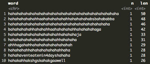
The longest “hahas” are 50, 48, and 46 characters long (H/T Pat, Dan, and Brad, respectively). Either something was very funny or someone is being very sarcastic.

Heading back to the first word count, after the “hahas,” I noticed quite a few bros’ names. It’s hard to know if someone is talking to or about someone else but let’s see if there is some sort of pattern between people who say each other’s names.

bros <- c((unique(data$Sender)), str_to_lower(unique(data$Sender)))
bros <- as.character(bros)
 
bro <- text %>%
  filter(word %in% bros) %>%
  group_by(Sender) %>%
  count(word, sort = TRUE)
 
broTable <- dcast(bro, Sender ~ word)
 
broTable[is.na(broTable)] <- 0
 
broTable$sum <- rowSums(broTable[, -1])
 
broTable <- arrange(broTable, desc(broTable$sum))

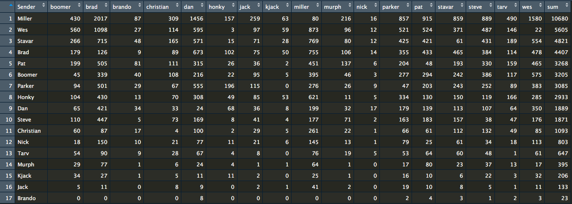
I created a table showing the sender and the number of times each bros’ name was said. While the table is a nice format to see the senders and each bro’s names, it’s a bit difficult to see any immediate trends even with sorting the sender by most messages sent. However, this is a nice opportunity to use a heat map.

ggplot(bro, aes(Sender, word)) +
  geom_tile(aes(fill = n), colour = "white") +
  scale_fill_gradient(low = "white", high = "red") +
  ylab("Bro")

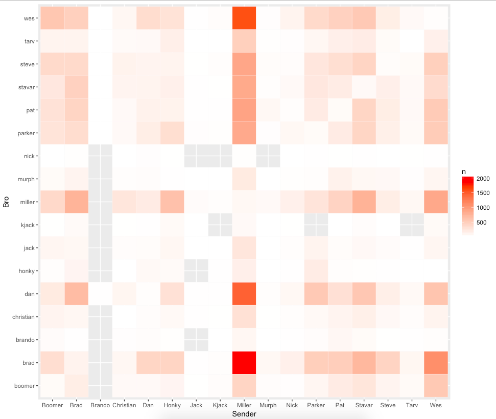
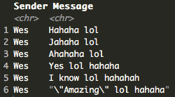
The heat map starts to tell the story a bit more. With the scale showing the brightest red as the most messages, it’s clear that Miller is mentioning Brad and Wes’ names quite a bit more than the others. This is falling in line since our first look at these messages showed Miller, Brad, and Wes send the most messages, equating to just under half of all the messages at 47%. We see the same pattern for Wes and Brad, telling me that a good portion of all these messages are Miller, Brad, and Wes talking with or about each other. Having known these three individuals, it all makes sense that there are so many “haha’s” since these are three of funniest people I know who enjoy making fun of each other and laughing. Wes has even been know to drop a few “hahaha lol’s” in his time.

data %>%
  filter(Sender == "Wes") %>%
  filter(str_detect(Message, "haha lol|lol haha")) %>%
  mutate(length = nchar(Message)) %>%
  arrange(length) %>%
  select(Sender, Message) %>%
  head()

While that was a bit more interesting, at least in my opinion, I still haven’t quite answered my original question. Since there are consistent spikes around February and March, the Super Bowl and March Madness, as well September, the start of the NFL Season, I suspect that most of these messages are sports related.

bros <- c((unique(data$Sender)), str_to_lower(unique(data$Sender)))
bros <- as.character(bros)

bruh <- filter(text, str_detect(text$word, "bruh"))
bruh <- as.character(unique(bruh$word))

ha <- filter(text, str_detect(text$word, "haha"))
ha <- as.character(unique(ha$word))

yea <- text %>%
  filter(str_detect(word, "yea")) %>%
  filter(!str_detect(word, "year")) %>%
  count(word, sort = TRUE)

yea <- unique(yea$word)

nums <- as.character(seq(1, 10))

fuck <- filter(text, str_detect(word, "fuck"))
fuck <- as.character(unique(fuck$word))

shit <- filter(text, str_detect(word, "shit"))
shit <- as.character(unique(shit$word))

randomWords <-
  c(
    "lol",
    "hill",
    "omitted",
    "image",
    "gif",
    "bros",
    "dude",
    "guy",
    "gonna",
    "gotta",
    "da",
    "bro",
    "im",
    "ya",
    "ass"
  )

myStopWords <- c(bros, bruh, ha, yea, nums, fuck, shit, randomWords)

textCleaned <- data %>%
  unnest_tokens(word, Message) %>%
  anti_join(stop_words) %>%
  filter(word %!in% myStopWords)

textCleaned$Date <- strptime(textCleaned$Date, "%m/%d/%y")
textCleaned$Time <- strptime(textCleaned$Time, "%I:%M:%S %p")
textCleaned$Time <- strftime(textCleaned$Time, format = "%H:%M:%S")
textCleaned$Month <- month(textCleaned$Date)

To start, I created my own stop words to add to the other list. I added any words that I felt didn’t really give an idea of what the conversation may have been about. Next, I cleaned up the data by correcting the date format. This allowed me to filter the data by month so that I could look specifically at February/March and September. Finally, I used dplyr and ggplot to reshape and visual the data into something more useful.

# Ferburary and March
textCleanedMarch <- textCleaned %>%
  select(Month, Sender, word) %>%
  filter(Month %in% c(2, 3))

marchViz <- textCleanedMarch %>%
  count(word, sort = TRUE) %>%
  filter(n > 225) %>%
  mutate(word = reorder(word, n)) %>%
  ggplot(aes(word, n)) +
  geom_col(fill = "royalblue4") +
  xlab(NULL) +
  coord_flip() +
  ggtitle("February & March")

# September
textCleanedSept <- textCleaned %>%
  select(Month, Sender, word) %>%
  filter(Month == 9)

septViz <- textCleanedSept %>%
  count(word, sort = TRUE) %>%
  filter(n > 150) %>%
  mutate(word = reorder(word, n)) %>%
  ggplot(aes(word, n)) +
  geom_col(fill = 'green4') +
  xlab(NULL) +
  coord_flip() +
  ggtitle("September")

grid.arrange(marchViz, septViz, ncol = 2)

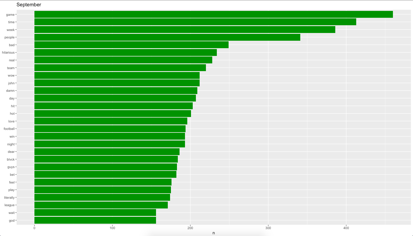
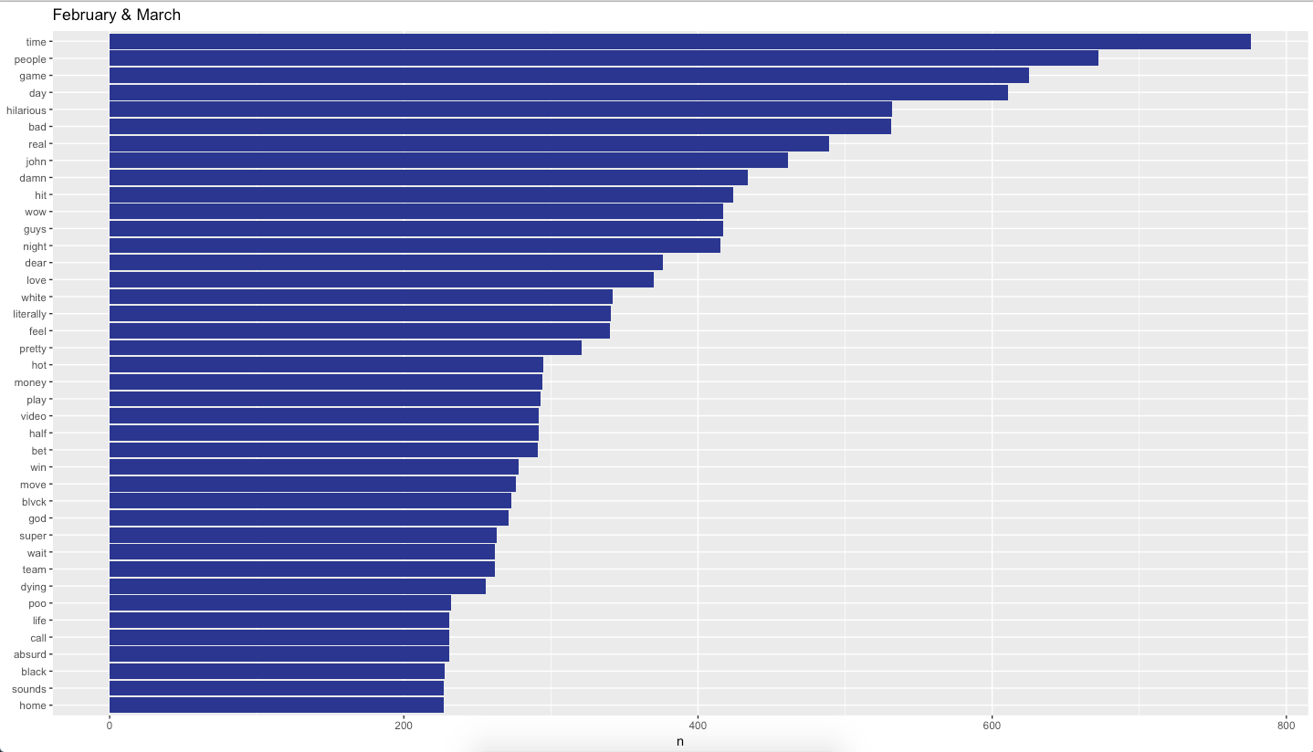
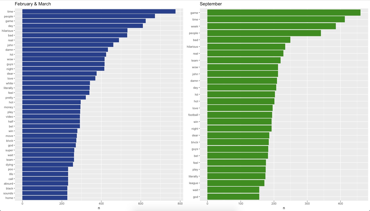
Right away, we see “game” listed at the top of February/March and September. For February/March, we see words such as “hit”, “money”, “play”, “bet”, “win” and “team”. I count twelve words of out of the top forty words in February/March, thirty percent, that are sports related. For September, “team”, “football”, “win”, “play”, and “league” make up eleven of the top twenty-eight words or thirty-two percent. To me, this is a pretty good indication that the conversations in February/March and September are indeed around Sports.

Overall, there’s nothing too groundbreaking found here. This is mainly a group chat of a bunch of guys being dudes, making fun of each other and talking sports. However, it is interesting that you can gain some insight into this chat with relative ease using the tools of the tidyverse.

Resources

• Text Mining with R
• ggplot2 Cheat Sheet
• R for Data Science – Data Visualisation