“Intermediate” Excel with R

Before finding my home at Fetch, I looked over tons of job descriptions. With everything becoming “data driven” these days, every role requires some familiarity with data and Microsoft Excel. I remember many of them requiring “Intermediate” skills, more specifically, pivot tables and Vlookup. While Excel is a solid starting point for organizing and manipulating data, nowadays there is so much data being collected making datasets bigger, more complex, and messier (see Pesky Dates Formats for the tip of the iceberg).

The bigger the data set, the less efficient Excel becomes, especially on a Mac. Handling larger datasets is where R and Python start to shine. This is part one of “Intermediate” Excel with R and Python, looking at pivot tables and Vlookup, starting with R.

Pivot Tables

Wikipedia describes a pivot tables as “a table that summarizes data in another table, and is made by applying an operation such as sorting, averaging, or summing data in the first table.” Pivot tables are quite helpful in breaking apart large datasets into smaller, more digestible pieces.

For the R side of things, the Tidyverse’s package, dplyr, makes data manipulation a breeze by using intuitive verbs that are somewhat like SQL. We’re going to keep the data set small just so we can see the functions working correctly but the same functions apply to a data set 10,000 times this size.

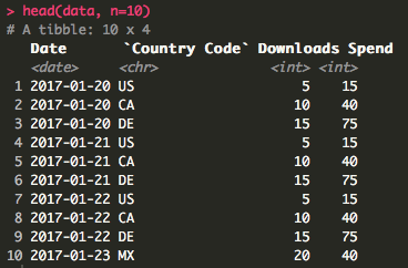
I’m going to be chaining functions together using the %>% operator, known as a “pipe.” To be honest, I don’t know exactly how chaining works behind the scenes. However, I find the code much more readable and I read the pipe as “then.”

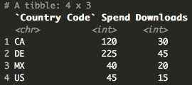
data %>%
  group_by(`Country Code`) %>%
  summarise(Spend = sum(Spend), Downloads = sum(Downloads))

Vlookup

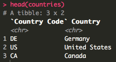
When I look at Vlookup now, I think of it as a join. In Excel, Vlookup can be tricky at first, especially when dealing with the array argument of the function. With R, I find things to be a bit easier. There are all kinds of joins but I typically use a left join to emulate Vlookup because it will force an NA when a match is not found. Here’s an example of looking up country names based on country codes.

For this to work correctly, there a couple of things to lookout for.

• The column header names for the join need to match or the join will fail.
• The lookup cannot have duplicates or the matching rows will duplicate on the main data set.

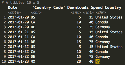
data <- left_join(data, countries, by = "Country Code")

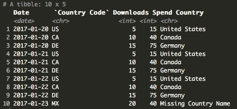
As you can see, we now have an NA for Country Code “MX” as it does not exist in the look up. There are numerous ways to handle NAs but here’s a quick way to change the NA to a string.

data$Country[is.na(data$Country)] <- "Missing Country Name"

However, we’re going to let the NA ride for now to show some of the functions dplyr has to deal with NAs.

Putting Them Together

Now that we have the full country names in our data set, let’s take our next example a bit further.

data %>%
  group_by(Country) %>%
  summarise(NumofCountry = n(),
            Spend = sum(Spend),
            Downloads = sum(Downloads),
            CPD = (Spend/Downloads)) %>%
  drop_na()

Here, we’ve added a couple of new things. We’ve added n() as NumOfCountry, which is returning the number of times each Country appears in the data set, similar to Count in Excel. We’ve also added CPD (Cost Per Download) as Spend/Downloads showing that we can also create calculated fields just like in Excel. Finally, we’ve included the drop_na() function to remove all of the NAs from the dataframe. We could also call drop_na() on a specific column to remove the NAs only for a particular column or remove drop_na() all together to have the NAs included.

Resources

There is a good chance there is a dplyr function for just about any data manipulation you may need to do. If you get stuck, you can always call the help menu on a function by doing something like ?summarise() or ?group_by().

Below, I’ve listed a link to a YouTube video of Data School going through some examples using dplyr and another YouTube video of Hadley Wickham using dplyr to clean up some data to then analyze. Both are great starting points for understanding exactly what dplyr can do and the flow of how to use this package to make your analysis smoother.

• YouTube – Data School – Hands on Dplyr Tutorial
• YouTube – Hadley Wickham – Whole Game
• Tidyverse – Dplyr GitHub
• Khan Academy – Intro to SQL

Code Snippet

library(tidyverse)
 
data <- read_csv("Excel Python or R Data.csv")
countries <- read_csv("Country Lookup.csv")
 
head(data, n=10)
head(countries)
 
data %>%
  group_by(`Country Code`) %>%
  summarise(Spend = sum(Spend), Downloads = sum(Downloads))
 
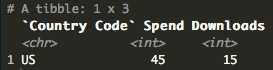
# Pivot - Spend and Installs by Country Code filter for US
data %>%
  filter(`Country Code` == "US") %>%
  group_by(`Country Code`) %>%
  summarise(Spend = sum(Spend), Downloads = sum(Downloads))
 
# Join to get full Country name
data <- left_join(data, countries, by = "Country Code")
 
# Replace NA with "Missing Country Name"
data$Country[is.na(data$Country)] <- "Missing Country Name"
 
# Pivot- Spend, Installs, CPD (Cost per Download) by full Country Name and Date
data %>%
  group_by(Country) %>%
  summarise(NumofCountry = n(),
            Spend = sum(Spend),
            Downloads = sum(Downloads),
            CPD = (Spend/Downloads)) %>%
  drop_na()
 
# help
?dplyr
?group_by
?summarise